Analyzing asset prices or future sales trends is extremely difficult, but advances have been made by adapting neural networks that have worked well in facial recognition.
In 2013, University of Chicago financial economist Eugene Fama shared the Nobel Memorial Prize in Economic Sciences for the analysis of asset prices.1 Fama, the father of the efficient market hypothesis, collaborated with Dartmouth College’s Kenneth French on research that identified three factors that explain a material portion of the variance in securities returns: market return, capitalization and book-to-market ratio.2 In 2015, Fama and French posited profitability and investment as additional factors.3
In parallel, New York University’s Stephen Brown used a tool known as principal component analysis (PCA) to develop predictive models to algorithmically identify orthogonal, or uncorrelated, factors in security returns.4
Both of these techniques — Fama’s use of arbitrage pricing theory (APT) and Brown’s PCA — attempt to unravel the complex currents of financial prices. Financial time series (sequences of market pricing data points in successive order) graphically resemble large zigzags distorted by small zigzags and may include stochastic drift, the change in the average value of a random process. Lurking beneath the surface of random-walking pricing data or, for that matter, seasonality-dependent retail product demand, patterns may exist that help predict future movements. In this article, we will explore some promising methods for extracting those patterns and gaining a deeper understanding of time series.
In asset management, research related to factors, either manually identified by financial theories or algorithmically extracted, are believed to be useful in asset allocation.5 Factor allocation offered asset managers more flexibility and opportunity than traditional allocation by asset class. These regression-based techniques found other uses as well, notably in retail, where trend and seasonality have been widely used to forecast product demand.
These methods employ linear features. In other words, the predicted time series consists of a sum of multiples of the features. APT makes the case that linear feature extraction is sufficient if the market is efficient and no arbitrage opportunities exist. And traditional retail forecasting models assume that future product demand is a function of measurable linear trends based on past demand. These two assumptions, however, are very context-specific and are often unrealistic. Intuitively, time series contain latent feature spaces — hidden variables that affect observable variables and explain the cross-section of time-series data, such as the performance of different assets or demand for products within a category.
For this reason, mathematical models that can capture nonlinear aspects of input data are necessary to improve forecasting performance. Nonlinear models can extract latent features and have potentially better explanatory power than linear functions.
Neural networks play a key role in nonlinear models and have been useful in almost all aspects of machine learning. Services like Amazon Forecast employ machine learning to predict future product demand, resource needs or division performance, using large datasets with irregular trends. The latest algorithms for retail forecasting combine time-series data such as price, discounts, web traffic and number of employees with independent variables like product features and store locations.
This article focuses on two increasingly important machine learning algorithms used to automate nonlinear feature extraction: variational autoencoders (VAEs) and generative adversarial networks (GANs) (see Figure 1). In exploring these algorithms, we will focus on pathbreaking research that’s been done in a field with fascinating similarities to financial or retail times series: image recognition.

Capturing Subtle Signals in Image Processing
Training neural networks isn’t easy; training them with financial data is an even greater challenge. Financial data has peculiarities: a low signal-to-noise ratio and behavior that varies over time. Although a neural network needs to be complex to capture both obvious and subtle data patterns, increasing complexity tends to produce models that perform poorly.
Algorithms that are nonlinear in terms of input data can extract subtle signals and generalize well to out-of-sample data. However, many neural network models cannot distinguish subtle signals from noise. This partly explains why neural network algorithms such as long short-term memory (LSTM) tend to overfit — not because there is too much noise but because the signal is too weak.
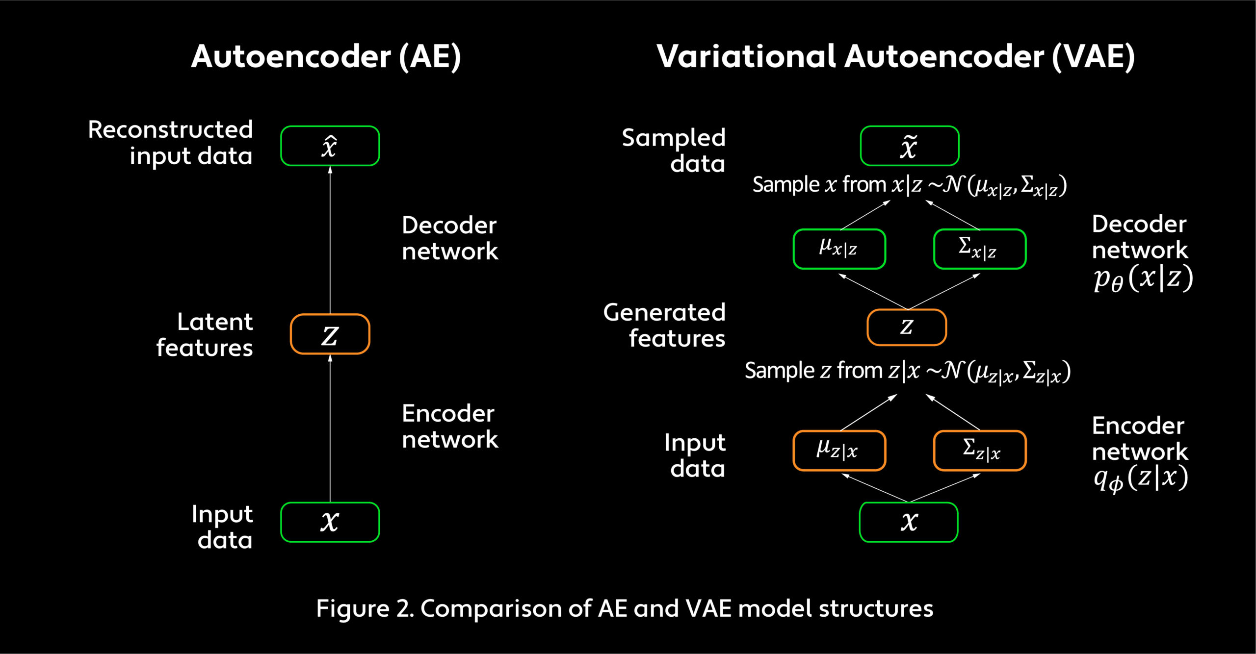
VAEs are neural networks that have been widely used in image recognition applications. A VAE is an unsupervised learning method that performs fast inference and learning using directed probabilistic models. It is, in fact, a probabilistic spin on the autoencoder (AE), which enables sampling from an unknown distribution to generate new data. Given input data, AEs learn through an encoder network that maps data to low-dimensional latent features and a decoder network that then transforms latent features to output data so that the reconstructed data is similar to the input data. VAEs work similarly, but their encoder and decoder networks operate probabilistically (see Figure 2).

In computer vision and image processing, feature extraction using VAEs has limitations. Latent features can correspond to facial attributes, orientation, lighting or other variations. In AEs, output data produces reconstructed images similar to input images. In VAEs, output data is probabilistically generated and output images may look different from input images. VAEs often fail to capture subtle features and can average out useful details, which they regard as noise. As a result, reconstructed pictures are usually blurry. This problem is related to the choice of error measures. VAEs commonly use pixel-based error measures, such as the mean squared error (MSE), which calculates the difference between each pixel in the original image and each pixel in the generated image, then takes the mean of the squared differences of those pixels. Small details may be harder to capture in error measures based on aggregation of such elementwise differences and will not be recognized by the encoder as an error. (Elementwise refers to operating on only one element of a matrix at a time.)

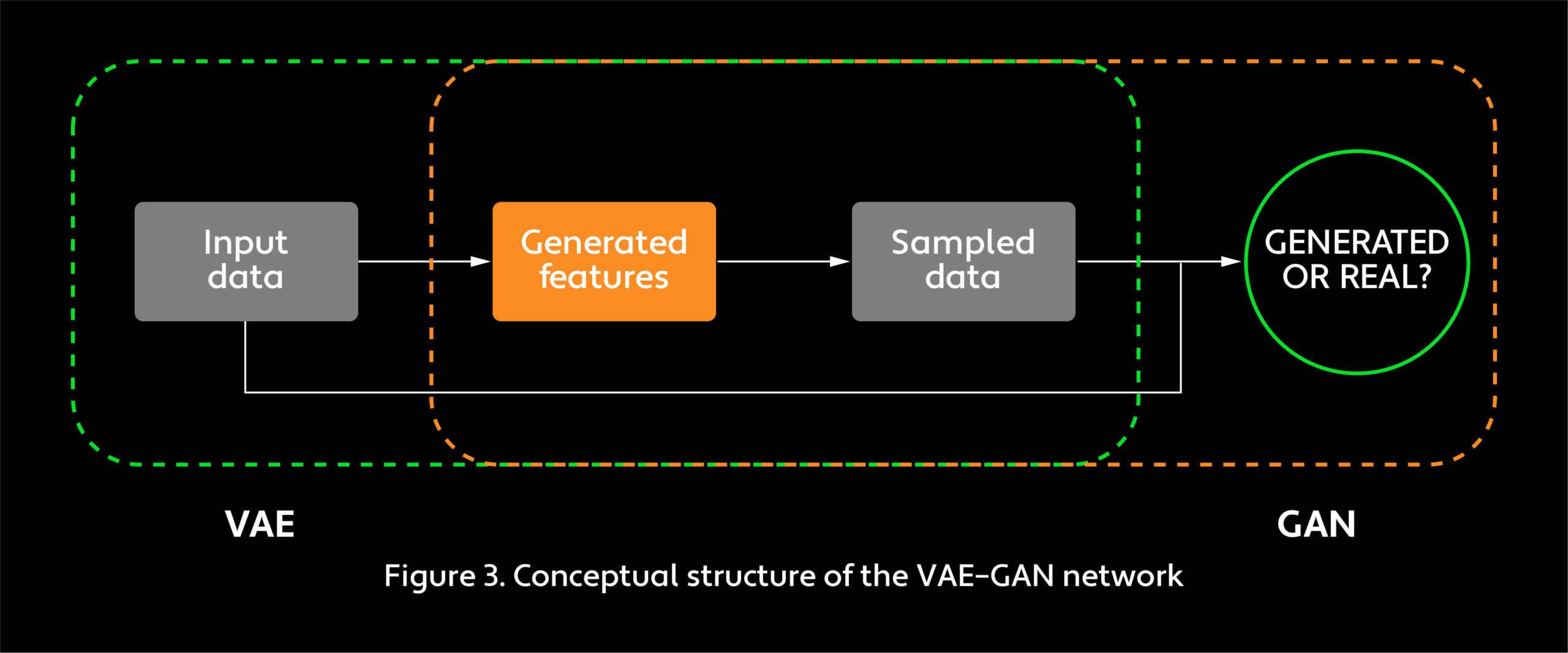
In 2016, Anders Larsen and his colleagues tackled the blurriness problem by bringing in a generative adversarial network, as shown in Figure 3.6 A GAN features two neural networks that compete with each other in a game, producing output data with the same statistics as the training data. Instead of using elementwise error measures, a GAN introduces measures that learn and improve during training. The logic is simple: If we have a complex neural network, an advanced error measure should be able to enhance the model’s performance.
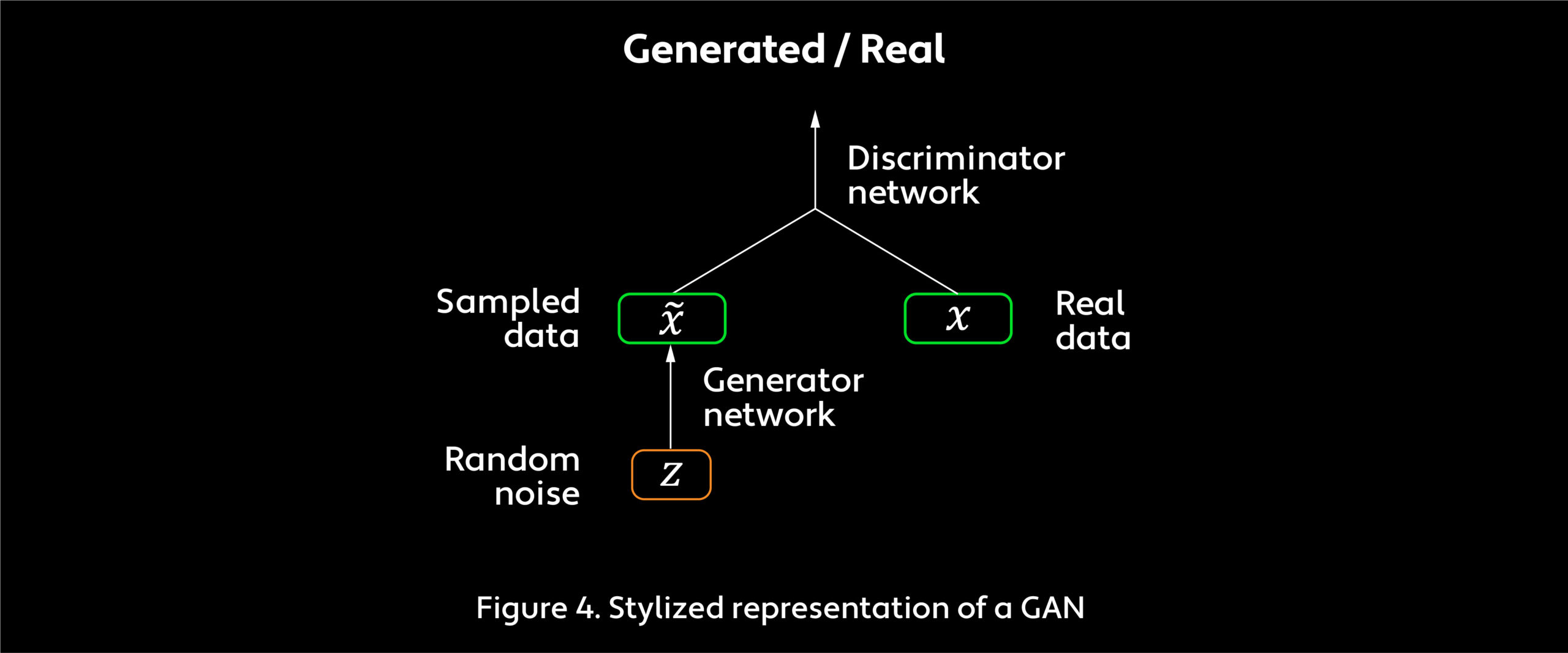
Larsen’s group combined the VAE decoder network and the GAN generator network into one component (see Figure 4). Like VAEs, GANs learn to generate samples that probabilistically resemble training data. Unlike VAEs, however, GANs assess the generator network by its performance competing against an opponent known as a discriminator network. Both the generator and the discriminator are neural networks. Training GANs is essentially a zero-sum game. The generator network aims to produce data that is indistinguishable from the original input data, while the discriminator network attempts to separate generated data from original data. As a seminal 2014 paper on GANs by Ian Goodfellow, a former researcher on the Google Brain project and today director of machine learning at Apple’s Special Projects Group, and his colleagues suggests,7 the generator network resembles a group of counterfeiters trying to produce fake currency without being detected, and the discriminator network acts like police tracking down fakes. Both the counterfeiters and the police improve during the game. What matters in the end are the counterfeiters, who have created an excellent way to print currency essentially indistinguishable from the real thing.

For facial recognition tasks, GANs significantly improve sample fidelity by simultaneously training a discriminator network that challenges the generator network with an increasingly higher standard. In this effort, GANs use another major loss function, called adversarial loss (AL), which seeks to minimize the divergence between two distributions.
GANs have since been adapted to a variety of tasks that involve unsupervised learning. Facebook, for instance, has worked with GANs to build learning models that incorporate properties like common sense.8
Applying VAE–GAN to Financial Time Series
Nonlinear feature extraction techniques like VAE and GAN have been successful in image processing, but can they be equally successful in the predictive challenges of a financial time series? To answer this question, we have to look into the similarities and differences in those two data types.
One of the most important similarities between processing image data and financial time-series data is the need for feature extraction. For example, to distinguish a human facial image with glasses from one without glasses, the machine has to extract that feature. Similarly, in order to flag anomalies such as potential financial fraud, the program has to recognize the presence of fraud. For predicting future demand for a product, the machine may have to extract features related to potential substitution for that product based on price.
Still, images and time-series data are fundamentally different data types. Image data is made up of a two-dimensional array of pixels, whereas time series involve values evolving over time. Both academic research and practical observations suggest that time-series data often contains multiple levels of cycles, seasonality and regimes. This necessitates different neural network structures for VAE and GAN. For image processing, a convolutional neural network (CNN) is more appropriate; for time series, LSTM may work more effectively.
Estimating posterior distribution is the most critical part of Bayesian inference — that is, the ability to update the probability of a hypothesis as more evidence accumulates. Posterior distribution is a way to summarize what we know about uncertain quantities, which can change with new data. In the past, expectation-maximization (EM) algorithms have been used for simple distributions and large datasets, and Monte Carlo (MC) sampling has been used for complex distributions and datasets of moderate size. However, many cases involve a complex posterior distribution and a very large dataset. In this case, EM cannot handle the complexity of the distribution and MC is too slow. This is when VAE becomes appealing. VAE’s neural network structure can handle complex posterior distributions and allows batch training for large datasets.9
VAE–GAN has many potential applications in time-series analysis. First, it can be a method to extract features, which can become inputs for predicting future returns and constructing signals. Second, the trained VAE on its own can be used to probabilistically sample from past financial time series, providing an alternative to backtesting methodology deterministically using historical single-trajectory data. Third, the trained GAN can be useful for evaluating new datasets. If a dataset contains new features, the discriminator network should be able to detect the change as discriminator error increases.
Earlier, we discussed how GAN, as an error measure, works in facial recognition by offering invariance under certain transformations, such as translation. This translational invariance — the ability to recognize an image even if it’s varied by, say, rotation — is also important to time-series analysis. Consider an algorithm that can reliably predict any 20 percent drop in sales of a particular product in the next five weeks. This is certainly useful, allowing the retailer to manage inventory and avoid a revenue hit. However, traditional pointwise error measures may consider the algorithms useless because they cannot pinpoint when the sales drop will occur. If GAN is used as an error measure instead, this type of algorithm can stand out in the training process.
For VAE–GAN to realize its potential, it is critical that we choose neural networks suitable for time series. One prominent characteristic of financial time series is cycling at multiple levels. For this reason, the architectures of recurrent neural networks (RNNs), such as LSTM and gated recurrent units (GRUs), are good candidates for VAE. Both LSTM and GRUs are designed to track data patterns with different frequencies over time; the main difference between them is the specific gates used in their architecture. In contrast to VAE, the discriminator network of GAN may require a different structure. To distinguish sampled time series from real ones, CNNs are potentially good options because they are adept at examining small features at each level of the neural network.
Financial time series normally display nonstationarity, or variance and autocorrelation that change over time. This poses a major challenge. For example, if today’s product price is set to be the regression target, then using a lag-1 product price can provide a good but useless fit. However, if percentage differences in product prices is used as the regression target, then the long-term trend will be lost. This nonstationarity issue is closely related to feature engineering. LSTM should take care of feature engineering during training, but this does not mean that manual preprocessing is unnecessary. The training model for feature engineering will drain information from the data and add noise to the process. If a feature is known to exist, it’s always better to incorporate it manually. However, too much feature engineering limits the model’s flexibility and makes it harder to find new features.
As with any neural network training, designing network structure (the number of nodes, layers in a neural network or activation functions) and tuning hyperparameters (learning rates, regularization weights) can be more art than science. But an experienced machine learning researcher can find the correct set of hyperparameters and unleash the power of VAE–GAN.
Conclusion
Generally, a time series is very difficult to accurately predict because the signal-to-noise ratio can be low and patterns change over time. Recent advances in machine learning related to VAEs and GANs have shown promising success in fields such as computer vision and image processing. Using these neural networks in tandem makes it possible to extract hidden features in image processing that seem to have a direct application to explanatory “hidden factors” in financial time-series data. VAEs and GANs may also have plausible applications in back testing, as well as in estimating the value-added of new datasets from an information theory standpoint. And VAEs and GANs are better suited to utilize certain invariance, cyclical and nonstationarity properties of financial time series, especially if users carefully choose compatible neural network architectures. Given the analogies between image processing and the flow of future financial prices or of product demand, sales and resource requirements, there’s currently a lot of hope invested in the potential of these advances in machine learning.
Michael Kozlov is a Senior Executive Research Director at WorldQuant and has a PhD in theoretical particle physics from Tel Aviv University.
Ashish Kulkarni is a Vice President, Research, at WorldQuant and has a master’s in information systems from MIT and an MS in molecular dynamics from Penn State University.
Bomin Jiang is an Intern at WorldQuant and PhD candidate at the Institute of Data, Systems and Society of MIT.
Flora Meng is an Intern at WorldQuant and PhD candidate in electrical engineering and computer science at the Laboratory of Information and Decision Systems of MIT.


